Tim Burton vs Steven Spielberg

IMDB ratings: Differences between directors
We are going to explore whether the mean IMDB rating for Steven Spielberg and Tim Burton are the same or not.
We write down the null and alternative hypotheses.
Null Hypothesis (H0) | The mean IMDB rating for Spielberg films = The mean IMDB rating for Burton films (Mean IMDB rating for Spielberg films - Mean IMDB rating for Burton films = 0) Alternative Hypothesis (H1) | The mean IMDB rating for Spielberg films != The mean IMDB rating for Burton films (Mean IMDB rating for Spielberg films - Mean IMDB rating for Burton films != 0 )
Load the data
movies <- read_csv(here::here("data", "movies.csv"))
glimpse(movies)
## Rows: 2,961
## Columns: 11
## $ title <chr> "Avatar", "Titanic", "Jurassic World", "The Aveng…
## $ genre <chr> "Action", "Drama", "Action", "Action", "Action", …
## $ director <chr> "James Cameron", "James Cameron", "Colin Trevorro…
## $ year <dbl> 2009, 1997, 2015, 2012, 2008, 1999, 1977, 2015, 2…
## $ duration <dbl> 178, 194, 124, 173, 152, 136, 125, 141, 164, 93, …
## $ gross <dbl> 7.61e+08, 6.59e+08, 6.52e+08, 6.23e+08, 5.33e+08,…
## $ budget <dbl> 2.37e+08, 2.00e+08, 1.50e+08, 2.20e+08, 1.85e+08,…
## $ cast_facebook_likes <dbl> 4834, 45223, 8458, 87697, 57802, 37723, 13485, 92…
## $ votes <dbl> 886204, 793059, 418214, 995415, 1676169, 534658, …
## $ reviews <dbl> 3777, 2843, 1934, 2425, 5312, 3917, 1752, 1752, 3…
## $ rating <dbl> 7.9, 7.7, 7.0, 8.1, 9.0, 6.5, 8.7, 7.5, 8.5, 7.2,…skim(movies)| Name | movies |
| Number of rows | 2961 |
| Number of columns | 11 |
| _______________________ | |
| Column type frequency: | |
| character | 3 |
| numeric | 8 |
| ________________________ | |
| Group variables | None |
Variable type: character
| skim_variable | n_missing | complete_rate | min | max | empty | n_unique | whitespace |
|---|---|---|---|---|---|---|---|
| title | 0 | 1 | 1 | 83 | 0 | 2907 | 0 |
| genre | 0 | 1 | 5 | 11 | 0 | 17 | 0 |
| director | 0 | 1 | 3 | 32 | 0 | 1366 | 0 |
Variable type: numeric
| skim_variable | n_missing | complete_rate | mean | sd | p0 | p25 | p50 | p75 | p100 | hist |
|---|---|---|---|---|---|---|---|---|---|---|
| year | 0 | 1 | 2.00e+03 | 9.95e+00 | 1920.0 | 2.00e+03 | 2.00e+03 | 2.01e+03 | 2.02e+03 | ▁▁▁▂▇ |
| duration | 0 | 1 | 1.10e+02 | 2.22e+01 | 37.0 | 9.50e+01 | 1.06e+02 | 1.19e+02 | 3.30e+02 | ▃▇▁▁▁ |
| gross | 0 | 1 | 5.81e+07 | 7.25e+07 | 703.0 | 1.23e+07 | 3.47e+07 | 7.56e+07 | 7.61e+08 | ▇▁▁▁▁ |
| budget | 0 | 1 | 4.06e+07 | 4.37e+07 | 218.0 | 1.10e+07 | 2.60e+07 | 5.50e+07 | 3.00e+08 | ▇▂▁▁▁ |
| cast_facebook_likes | 0 | 1 | 1.24e+04 | 2.05e+04 | 0.0 | 2.24e+03 | 4.60e+03 | 1.69e+04 | 6.57e+05 | ▇▁▁▁▁ |
| votes | 0 | 1 | 1.09e+05 | 1.58e+05 | 5.0 | 1.99e+04 | 5.57e+04 | 1.33e+05 | 1.69e+06 | ▇▁▁▁▁ |
| reviews | 0 | 1 | 5.03e+02 | 4.94e+02 | 2.0 | 1.99e+02 | 3.64e+02 | 6.31e+02 | 5.31e+03 | ▇▁▁▁▁ |
| rating | 0 | 1 | 6.39e+00 | 1.05e+00 | 1.6 | 5.80e+00 | 6.50e+00 | 7.10e+00 | 9.30e+00 | ▁▁▆▇▁ |
# We use the duplicated() function to identify duplicates, and find that there are none
summary(duplicated(movies))
## Mode FALSE
## logical 2961director_rating <- movies %>%
filter(director %in% c("Steven Spielberg","Tim Burton"))
# We summarise data using mean and CI functions
director_rating2 <- director_rating %>%
group_by(director) %>%
dplyr::summarise(mean_rating = mean(rating),
uci_rating = CI(rating)[1],
lci_rating = CI(rating)[3])
# We use geom_errorbar and geom_react in order to reproduce the graph
ggplot(director_rating2, aes(x = mean_rating, y = reorder(director, mean_rating), colour=director)) +
geom_point(size=5, show.legend = FALSE)+
# We use geom_rect to draw overlapping sections
geom_rect(aes(xmin=uci_rating[2], xmax=lci_rating[1], ymin=-Inf, ymax=Inf), colour = "light grey", alpha = 0.2)+
# We use geom_errorbar to draw CI intervals
geom_errorbar(aes(xmin = lci_rating, xmax = uci_rating), size=1.3, width=.05, show.legend = FALSE)+
geom_text(aes(label = round(lci_rating,2), x = lci_rating), size= 4.5, vjust = -1, colour ="black")+
geom_text(aes(label = round(mean_rating,2), x = mean_rating), size= 6, vjust = -1, colour ="black")+
geom_text(aes(label = round(uci_rating,2), x = uci_rating), size= 4, vjust = -1, colour ="black")+
labs(x="Mean IMBD Rating",
y= "", title= "Do Spielberg and Burton have the same mean IMDB ratings?",
subtitle= "95% confidence intervals overlap")+
theme_bw()+
NULL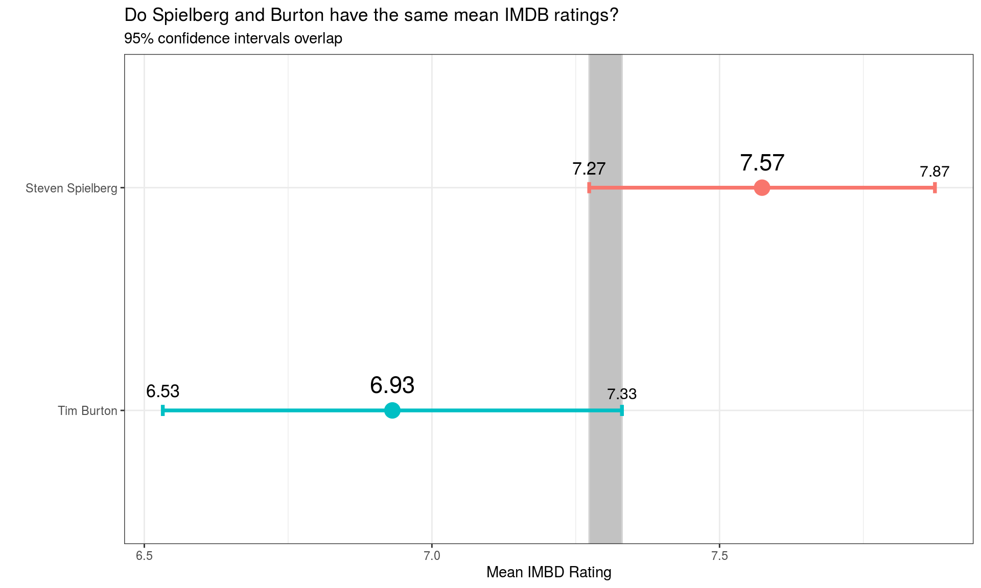
In addition, we run a hypothesis test using both the t.test command and the infer package to simulate from a null distribution, where we assume zero difference between the two.
Hypothesis testing
director_rating <- movies %>%
    filter(director %in% c("Steven Spielberg","Tim Burton")) # select directors
  t.test(rating~director, director_rating)
##
## Welch Two Sample t-test
##
## data: rating by director
## t = 3, df = 31, p-value = 0.01
## alternative hypothesis: true difference in means is not equal to 0
## 95 percent confidence interval:
## 0.16 1.13
## sample estimates:
## mean in group Steven Spielberg mean in group Tim Burton
## 7.57 6.93First, we use the t.test to calculate the p-Value. We conclude that there is a statistically significant difference in means, since our p-value is 0.01 and hence |p|<a (where a=0.05) (or |t| > 2.00). Therefore, we reject the null hypothesis. Now we run the simulation with the infer package:
set.seed(1234) # We set a specific seed value

# We run a simulation with infer package

director_hypothesis_test<- director_rating %>%

  specify(rating ~ director) %>%

  # Here, `hypothesize` is used to set the null hypothesis as a test for independence, i.e., that there is no difference between the two population means.
  hypothesise(null="independence") %>%
  # The `type` argument within generate is set to permute, which is the argument when generating a null distribution for a hypothesis test.
  generate(reps=1000, type="permute") %>%
  #calculate the observed difference in means with bootstrap
  calculate(stat="diff in means",order = c("Steven Spielberg","Tim Burton"))


diff_rating <- director_rating %>%
  specify(rating ~ director) %>%
  calculate(stat = "diff in means", order = c("Steven Spielberg","Tim Burton"))
#get p_Value through infer package
director_p_value <- director_hypothesis_test %>%
    get_p_value(obs_stat = diff_rating[1,1], direction = "both")

kbl(director_p_value,col.names=c("p-value"), caption="Simulation-based null distribution using the 'infer' package") %>%
kable_styling()| p-value |
|---|
| 0.008 |
Again, on the basis of this simulation-based hypothesis test we reject the null hypothesis stating that there is no difference in means of IMDB rating for Spielberg films and for Burton films as the p-Value is smaller than the alpha value (0.05). Therefore there is statistically significant difference between the mean ratings of the films of the two film directors. We visualise the simulation-based null distribution:
#We calculate CI using infer package
director_percentile_ci <- director_hypothesis_test %>%
get_confidence_interval(level = 0.95, type = "percentile")
#We show a plot with shaded confidence interval using infer package
director_hypothesis_test %>% visualise() +
shade_confidence_interval(endpoints = director_percentile_ci, size=0.4, color= "yellow", fill="light yellow") +
shade_p_value(obs_stat = diff_rating, direction = "both", size=1.1) +
labs(title = "Are Spielberg and Burton Equally Good Directors?",
subtitle="Simulation-based null distribution: the p-value (red) lies well outside the null distribution (yellow), allowing us to reject the null hypothesis", x="Difference in Mean IMDB Rating Between Directors", y="Count")+theme_fivethirtyeight() + theme(axis.title = element_text()) + scale_x_continuous(breaks=seq(-1.0, 1.0, by = 0.1), limits=c(-1.0,1.0))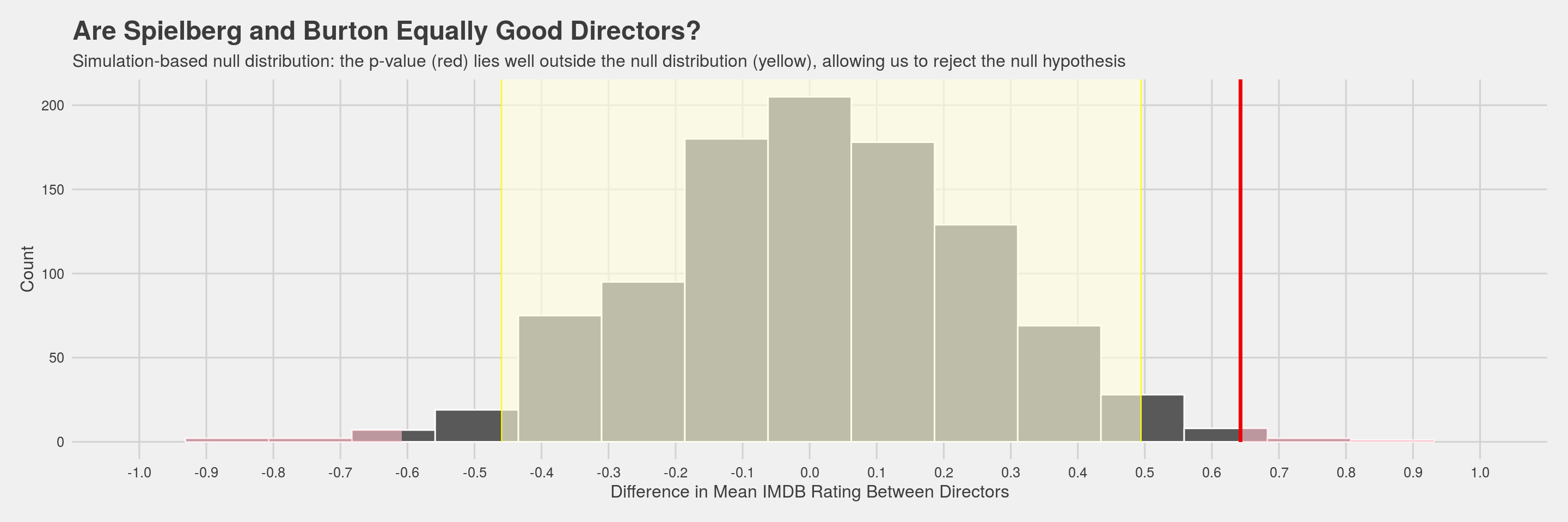 In the graph it is shown that the p-value is outside of the 95% confidence interval (alpha = 0.05). We therefore reject the null hypothesis (H0) that there is no difference in the mean IMDB ratings of the films of Tim Burton and Steven Spielberg.