Create a plot

We Calculate the average net approval rate (approve-disapprove) for each week since Trump got into office. We plot the net approval, along with its 95% confidence interval.

#we create a week identifier for each week and group by the week identifier and year the week falls under, before taking a mean of the net approval ratings within each week

net_approvals <- approval_polllist %>% 

  filter(subgroup=="Voters") %>% 
  
  mutate(net_approval=approve-disapprove) %>% 
  
  mutate(week_number=isoweek(enddate)) %>% 
  
  mutate(year=year(enddate)) %>% 
  
  group_by(year, week_number) %>% 
  
  summarise(week_net_approval=mean(net_approval,na.rm=TRUE),sd_approval=sd(net_approval,na.rm=TRUE),count=n(),t_critical=qt(0.975,count-1),se_approval=sd_approval/sqrt(count),margin_of_error=t_critical*se_approval,approval_low=week_net_approval-margin_of_error,approval_high=week_net_approval+margin_of_error)

ggplot(net_approvals, aes(x=week_number,y=week_net_approval)) + geom_point(aes(colour=as.factor(year)), size=0.6) + geom_line(aes(colour=as.factor(year))) + facet_wrap(~year) + theme(legend.position="none") + labs(x="Week of the year",y="Average Net Approval (%)",title="Estimating Net Approval (approve-disapprove) for Donald Trump",subtitle="Weekly average of all polls") + geom_hline(yintercept=0, colour="orange") + scale_y_continuous(limits=c(-22.5,7.5), breaks=seq(-20,7.5,2.5)) + scale_x_continuous(breaks=c(0,13,26,39,52)) + geom_ribbon(aes(ymin=net_approvals$approval_low, ymax=net_approvals$approval_high, colour=as.factor(year), fill=as.factor(year)),alpha=0.1)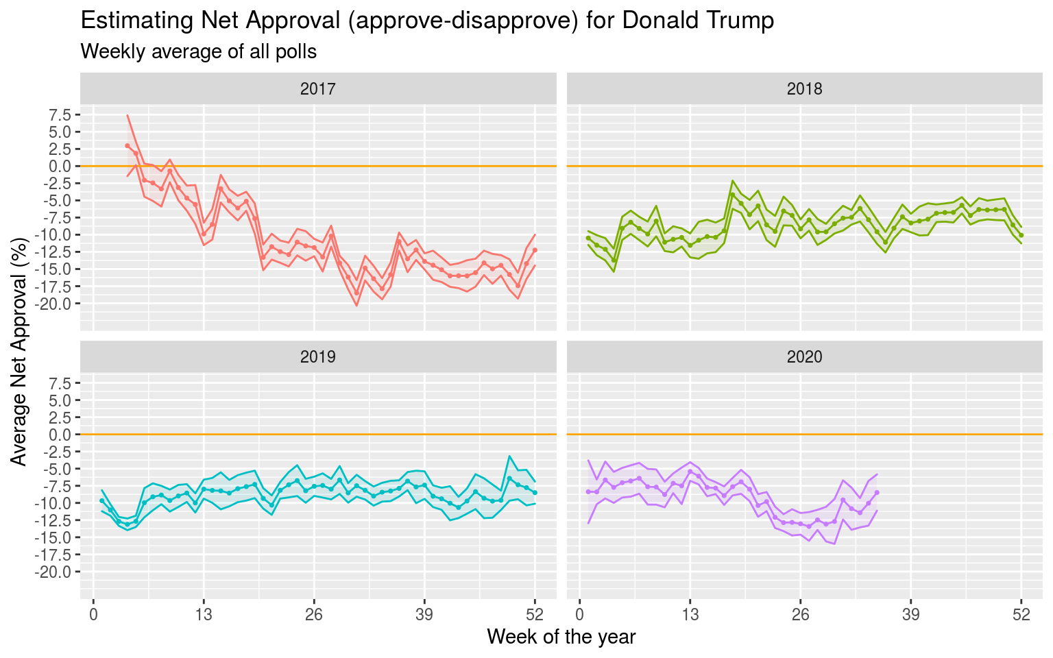

Compare Confidence Intervals

We compare the confidence intervals for week 15 (6-12 April 2020) and week 34 (17-23 August 2020).

CI_comparison <- net_approvals %>% 
  filter(year==2020,week_number %in% c(15,34))
         
CI_comparison %>% 
  select(c(1,2,9,10)) %>% 
kbl(col.names=c("Week Number","Year","Net Approval: Lower Limit (%)","Net Approval: Upper Limit (%)")) %>%
kable_styling()

Across both confidence intervals, Trump’s net approval rating is negative, but in Week 15, the lower bound is greater than even the upper bound in Week 34. The 95% confidence interval is also considerably wider in Week 34 than in Week 15 (1.48 in Week 15, versus 3.78 in Week 34). This implies both that the amount of variation in Trump’s net approval ratings generated by polls in Week 34 is considerably greater than that generated by those earlier in the year and that his mean net approval has unambigiously fallen. The observed decline in net approval is to be expected, since Trump’s handling of the COVID-19 pandemic has been sloppy and the US has one of the most severe outbreaks of the virus, given poorly enforced and coordinated federal measures and weak norm compliance.

The increase in the size of the confidence interval suggests both that poll sample sizes may have fallen (increasing variability) and that the events of the summer have increased uncertainty over Trump’s popularity, reflected by greater variation in popularity ratings between polls than earlier in the year, when polls were more consistent with one another. This increased variation between polls may be caused by differences between samples used by polls, such as between certain states or counties. This is an especially likely cause since the COVID-19 pandemic has had heterogeneous effects across the country and Trump’s approval rating is likely to depend on the perceived success of measures in voters’ home states. Consequently, cross-country approval polls in Week 15 are likely to be far more consistent with one another than those taken in Week 34, resulting in wider 95% confidence intervals in the latter period.